This model is a proof-of-concept example for combining FlexSim's GIS features with the power of mixed integer programming in python. The model simulates a distribution network of 'factories' (red icons) and 'warehouses' (blue icons). The factories produce the product you are selling, and then distribute the product to various warehouses in the network.
Every day, each warehouse generates a random demand for the product. Once demand from each warehouse is known, the 'demand dispatcher' must determine which factory should produce and ship how much of the product to each warehouse, fulfilling all warehouses' demands at minimum total cost. Each factory has a maximum daily capacity of production and a per-unit cost of production. In addition, shipping costs must be taken into account from each factory to each warehouse. Given these factors and constraints, the problem of optimal dispatching boils down to the well-known min cost flow problem in optimization.
I've created a simple python script that uses cvxpy to solve this min cost flow problem as a mixed integer program. The MIP is not exactly the same as the standard min cost flow problem, since total factory capacity may be more than total warehouse demand, and I'm using integer instead of continuous variables. Nevertheless, it is sufficient to demonstrate the capability.
The Warehouse process flow generates daily demand for each warehouse and pushes it to a shared Demand list. The DemandDispatcher then pulls demand from the list, and marshals capacity, demand, and cost data into parameters that can be passed to python. Then it evaluates getMinCostFlow label on the process flow, passing those parameters in. The label is configured to connect to the getMinCostFlow function defined in the MinCostFlow.py module. This function formulates the MIP with cvxpy, solves the program, and then returns the optimal shipping quantities for each factory-warehouse pair, returning control back to FlexSim.
Once the shipping quantities have been resolved, the DemandDispatcher process flow creates and labels 'Trucks' that are sent to each warehouse. Note that this travel mechanism is purely for animation purposes, letting you visualize how much product is being sent from factories to warehouses each day. Potential additions to this model could use inventory management strategies, simulating randomized lead times, etc.
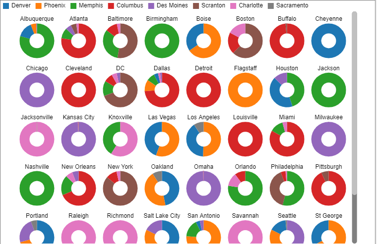
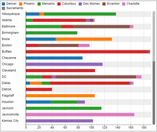
I've added several dashboards that show the cumulative average breakout for each warehouse of which factories supply that warehouse, as well as the cumulative average breakout for each factory of which warehouses that factory supplies. I've also added costing measures for the warehouses and factories.
Some interesting insights that can be gleaned from this model are how shipping vs. production costs affect the balance of which factories will ship to which warehouses. For example, if your shipping costs are low relative to your production costs, then the min cost flow algorithm will push production to factories that are the lowest cost to produce, even if they are far away from the destination warehouse. High production cost factories are consequently relegated to little if any production. However, if shipping costs are high, the algorithm will localize production to the factories nearest their respective warehouses.
In order to run this model, you need python properly configured, including:
- Install one of these python versions: 3.7, 3.8, 3.9, 3.10
- Install the cvxpy and cvxopt packages: python -m pip install cvxpy cvxopt
- Make sure the python directory is part of your PATH environment variable
- Configure your Global Preferences (the Code tab) to use the associated python version.
This model was built in FlexSim 22.1.
